

1. Introduction
2. Theoretical Background
2.1 Frequency-dependent Attenuation and Propagation Velocity in Saturated Soils
2.2 Characteristic Frequency and Hydraulic Conductivity of Soils
3. Test Setup
4. Sample Preparation
5. Determination of the Characteristic Frequency
(1) Technique A (Quality Factor Based Measurements)
(2) Technique B (Wave Velocity Based Measurements)
6. Test Results
6.1 1/Q and Velocity Spectra for Dry Specimens
6.2 1/Q and Velocity Spectra for Saturated Sand Specimens
6.3 1/Q and Velocity Spectra for Saturated Sand and Bentonite Mixture
6.4 AC and DC Hydraulic Conductivity
7. Conclusions
1. Introduction
In the area of seismic exploration, it is difficult to control the frequency of seismic waves, but it is relatively easy to generate a high amplitude wave that can propagate significant distances through the ground. Some actuators may generate vibrations with some degree of the frequency control, but the range of their operating frequency is limited. If one switches to acoustic wave sources, one loses the strength of excitation but obtains a better control on the frequency, and one can study frequency dependent soil properties such as the hydraulic conductivity of soils.
The frequency dependence of the propagation velocity and attenuation of waves in sandy sediments have been extensively investigated by many researchers (Nolle et al., 1963; Hamilton, 1972; Hamdi and Smith, 1982; Hickey and Sabatier, 1997; Velea et al., 2000; Stoll, 2002; Williams et al., 2002; Buckingham, 2004; Lu et al., 2004; Emerson and Foray, 2006; Zimmer et al., 2007a, 2007b; Lee et al., 2007). Worth noting down this study, Prasad and Meissner (1992) reported the variation of propagation velocity and attenuation of high frequency waves for different grain size, shape, porosity, density, and static frame compressibility of dry and water-saturated sands subjected to varying confining pressures.
Biot (1956a, 1956b)’s pioneering work showed that the elastic excitation of saturated soils causes out-of-phase vibration of solid particles and pore water. The amplitudes and phases of motion for these two constituents, therefore, may not be the same. Ultimately, when the excitation frequency causes the maximum difference in phases of motion between the two constituents, the attenuation of the acoustic wave reaches its peak. This frequency is known as the “characteristic frequency”. On the other hand, dynamic water flow at the surface of solid grains is accompanied due to the differences in the amplitude of motion between solid particles and pore water. Therefore, the characteristic frequency implicitly includes the hydraulic properties of porous media, and a proper coupled analysis may enable the estimation of the hydraulic conductivity of soils using the characteristic frequency. The relationship between the characteristic frequency and the hydraulic conductivity is extensively used in Geophysics area such as shown in Buckingham (2004), Diallo et al. (2003), Dvorkin and Nur (1993), Stolle (2002) and Yamamoto (2003).
This study adopted Biot’s coupled theory of mixtures to explore the possibility of estimating the hydraulic conductivity of soils often considered as unconsolidated formations in Geophysics. The characteristic frequency of artificially prepared specimens was measured using two acoustic techniques: (1) attenuation-based measurements and (2) velocity-based measurements. As a consequence, more reliable and repeatable characteristic frequencies are obtained.
2. Theoretical Background
2.1 Frequency-dependent Attenuation and Propagation Velocity in Saturated Soils
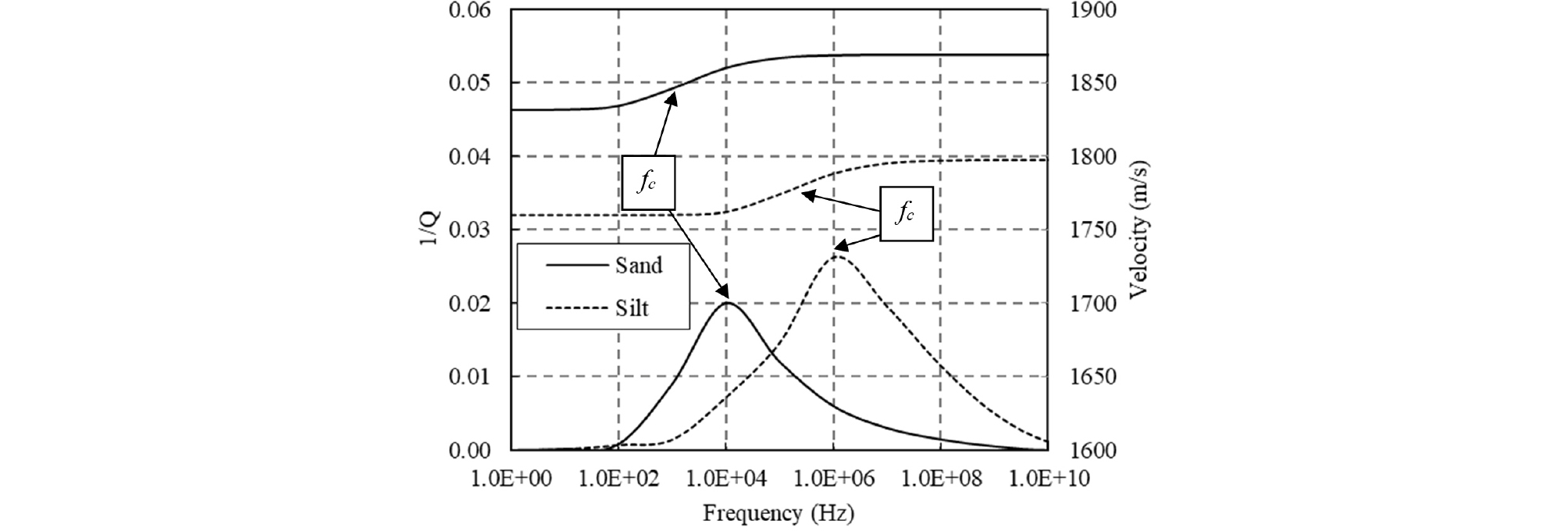
The propagation mechanism of P-waves in solid media varies with its excitation frequency. According to Hughes et al. (2003), the motion of the solid skeleton is dominated by the viscous coupling of the pore fluid and the solid skeleton in the low frequency range and by the inertial coupling of these two constituents in the high frequency range. At a specific frequency called the characteristic frequency, the effect of viscous coupling and inertial coupling is about the same, showing distinctively different behavior before and after this frequency for porous materials. This frequency response essentially brings out a bell shaped quality factor distribution and two different propagation velocity distribution before and after the characteristic frequency, as shown in Fig. 1. For two different soils, characteristic frequencies are different, and two different response curves are obtained.
From Fig. 1, the characteristic frequency is determined from the point where the highest 1/Q (inverse quality factor) is observed from the curve of 1/Q plotted versus frequency; alternatively, it can be determined from the inflection point of the curve of P-wave velocity vs. frequency (also shown in Fig. 1). One of the unique traits of the characteristic frequency is its relation to the hydraulic conductivity of soils. As shown in Fig. 1, a higher characteristic frequency is observed in soils of lower hydraulic conductivity (silt) than in soils of higher hydraulic conductivity (sand). Therefore, it is anticipated that the characteristic frequency may have potential to estimate the hydraulic conductivity of soils.
2.2 Characteristic Frequency and Hydraulic Conductivity of Soils
According to Biot (1956a, 1956b, 1962), the relationship between the characteristic frequency and hydraulic conductivity of soils is expressed as follows:
where, n is the porosity, k is the hydraulic conductivity in m/sec, g is gravity in m/sec2, and fc is the frequency in hertz. Eqn (1) is a derivation based on linear elastic wave propagation theories for water saturated media which assume that the pores are uniform in size and interconnected, the wave length is much longer than the grain size, and that Darcy’s law is valid. More sophisticated models have also been proposed by other researchers who consider more realistic macroscopic flow mechanisms, pore shapes, and possible micro pores in solid particles. Some examples include the squirt flow mechanism (Dvorkin and Nur, 1993; Dvorkin et al., 1994 and 1995; Yamamoto, 2003), modified BISQ (Biot and Squirt flow) mechanism (Diallo et al., 2003), and mesoscopic flow mechanism (Pride and Berryman, 2003b; Wei and Muraleethran, 2006). This paper adopted equation (1) for simplicity. For a more extensive discussion of P-wave propagation and the possible existence of additional P-waves (second and third dilatational waves) in geo-materials, the reader is referred to Lopatnikov and Cheng (2004).
3. Test Setup
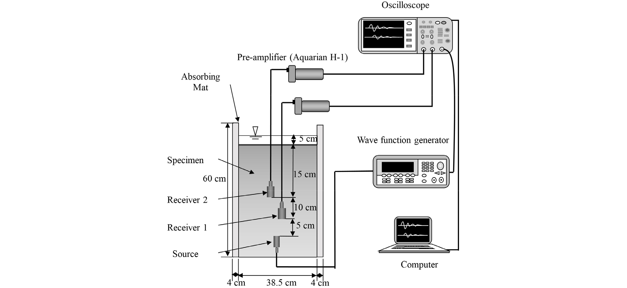
The test setup in this study was similar to the one presented by Song et al. (2008), but this study used a smaller diameter acoustic source (Aquarian Audio Products, Hydrophone H-1) to create more uniform far field conditions. A function generator (Agilent Technologies, 33220A) was used to supply a single cycle sinusoidal wave with a 0° phase angle. Two receivers (Aquarian Audio Products, Hydrophone H-2) with built-in pre-amplifiers were used to receive the P-wave signals, which were then recorded by a digital oscilloscope (Agilent Technologies, DSO 3202A) using a 1G Sa/s sampling rate. The frequency response of the acoustic source and receivers was not known; therefore, it was checked by testing the system with dry sand. The result is shown in “Test Results”, and a near flat frequency response is observed. The travel time was computed by comparing the arrival times of peak amplitudes with a source-to-receiver distance of 5 cm and 15 cm. To reduce the coupling effect and to guarantee the accurate orientation of the transducers, the vertical and horizontal orientation of the transducer was double-checked before measurements were taken. However, the coupling effects due to micro-mechanical quantities, such as differing particle sizes and internal stress conditions, were disregarded in this study. To minimize the reflection of waves, sound absorbing mats (Home Trends, 887V-W) were placed around the side walls of the test box. Additionally, the distance between the top of the soil and the receiver was kept at 20 cm to reduce the effect of reflected P-waves from the soil-water interface at the top. However, a quantitative evaluation of the effects of reflection could not be made. The overall test setup is schematically shown in Fig. 2.
4. Sample Preparation
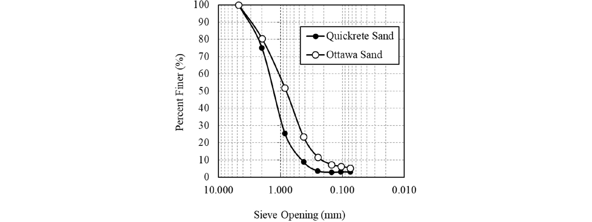
Four different soil samples were used in this study as shown in Table 1. QUIKRETE® No. 1152 (QUIKRETE®, Georgia) and Ottawa Sand C-109 (U.S. Silica Co. Ottawa, Illinois) were used for the sand specimens and labeled SQ (Sand-QUIKRETE) and SO (Sand-Ottawa), respectively. The gradation curves for SQ and SO soils are shown in Fig. 3.
Table 1.
General properties and components of test samples
| Name | Mixing ratio by Wt. | γd (t/m3) | w (%) | n | |
| Sand (%) | Bentonite (%) | ||||
| SQ | 100 | 0 | 1.65 | 22.68 | 0.375 |
| SO | 100 | 0 | 1.70 | 20.98 | 0.357 |
| SQB1 | 99 | 1 | 1.73 | 19.81 | 0.333 |
| SOB1 | 99 | 1 | 1.74 | 19.88 | 0.345 |
To control the hydraulic conductivity of the specimens, 1% (by weight) of sodium bentonite (BARA-KADE Standard, BPM Minerals, LLC, Lovell, Wyoming; Gs=2.7, Min 67.5% pass through #200 sieve) was mixed with the QUIKRETE® No. 1152 and named SQB1. The following is the step-by-step procedure used for preparing SQB1 in this study:
1. The required materials for preparing the sand and bentonite mixture were weighed in the following amounts: Total weight of dry sand (95.4 kg), bentonite (0.954 kg), and water (22.16 kg) according to predetermined amounts (for 1% bentonite content). From the premeasured saturated water content of this sample (23%), the authors determined the required amount of water to be 22.16 kg (23% of the total weight of the sand and bentonite mixture, 96.354 kg). A mixture with a higher water content was tried but discarded because it caused free water at the surface of the specimen in which an undetermined quantity of suspended bentonite particles was observed.
2. Three identical batches of the material mixtures were prepared to ensure a more even distribution of sand and bentonite throughout the entire specimen. For the first layer, the bentonite (0.318 kg) was poured into the sand (31.800 kg) in the mixing container (Sterilite, 18 Gallon, 1815).
3. The bentonite and sand were then dry-mixed using the researcher’s hands in the container.
4. 5.909 kg of water was then poured into the mixture, which is 80% of the total required amount of water for the first layer (the total amount of water for the first layer is 7.386 kg). Then, the material was again mixed by the researcher’s hands for about 3 minutes until a uniform mixture was observed.
5. After visual uniformity was achieved, the mixing was continued for another five minutes using a rotary mixer (Makita Power Drill, 6302H and Homax Mixing Blade, 69170).
6. The bentonite, sand, and water mixture was carefully poured from the mixing container into the acoustic test box using a small shovel to prevent material separation.
7. To completely soak the specimen, the remaining 1.48 kg (20%) of water was added.
8. Any free water was removed from the surface of the soil.
9. Steps 2-8 were repeated for the second and third layers.
10. After finishing the preparation of the sand/bentonite mixture, the researchers applied an additional 4.5 kg of water to the top surface of the soil specimen to guarantee that the specimen to maintain saturation even after the bentonite particles absorbed the water.
SOB1 was prepared in the manner indicated above; however, SQ and SO were both prepared without adding bentonite to the mixture in the above steps.
5. Determination of the Characteristic Frequency
(1) Technique A (Quality Factor Based Measurements)
Technique A is based on the frequency dependency of the inverse quality factor, for which the characteristic frequency is determined from the peak point in Fig. 1. To measure the inverse quality factor, amplitudes of received acoustic signals from two hydrophones at two different predetermined distances from the source were compared. The frequency was swept from 1 kHz to 10 kHz with an interval of 500 Hz for sand specimens and 1 kHz to 25 kHz with an interval of 500 Hz for sand and bentonite mix specimens. Measured amplitudes from the different frequencies were used for computing the inverse quality factor as follows (Kim, 2010; Raji and Rietbrock, 2013):
where, A1 is the amplitude measured from a receiver with a distance r1 from the source; A2 is the amplitude measured from a receiver that has distance r2 from the source; (r1 – A2) is the difference in distance between the two receivers; c is the speed of sound in the porous media; and f is the frequency of received signal.
(2) Technique B (Wave Velocity Based Measurements)
Technique B is based on the frequency dependency of wave velocities. While the frequency was being swept, the velocity was computed from the measured travel time. The characteristic frequency was obtained from the inflection point of the velocity vs. frequency curve. Zero crossing time was initially employed, but the peak amplitude time technique was eventually adopted because it resulted in more consistent readings. Moreover, to reduce the effect of ambient noise, a digital filtering technique with 5, 10, 15, 20, 25, and 30 kHz high pass digital cut-offs was used depending on the noise conditions. In order to minimize the effect of random noise, an ensemble average of 128 signal sets was used.
From the measured velocity spectra, the maximum of the inverse quality factor was also evaluated using a Biot-Gassmann-asymptotic relationship as proposed by Santamarina et al. (2001) as follows:
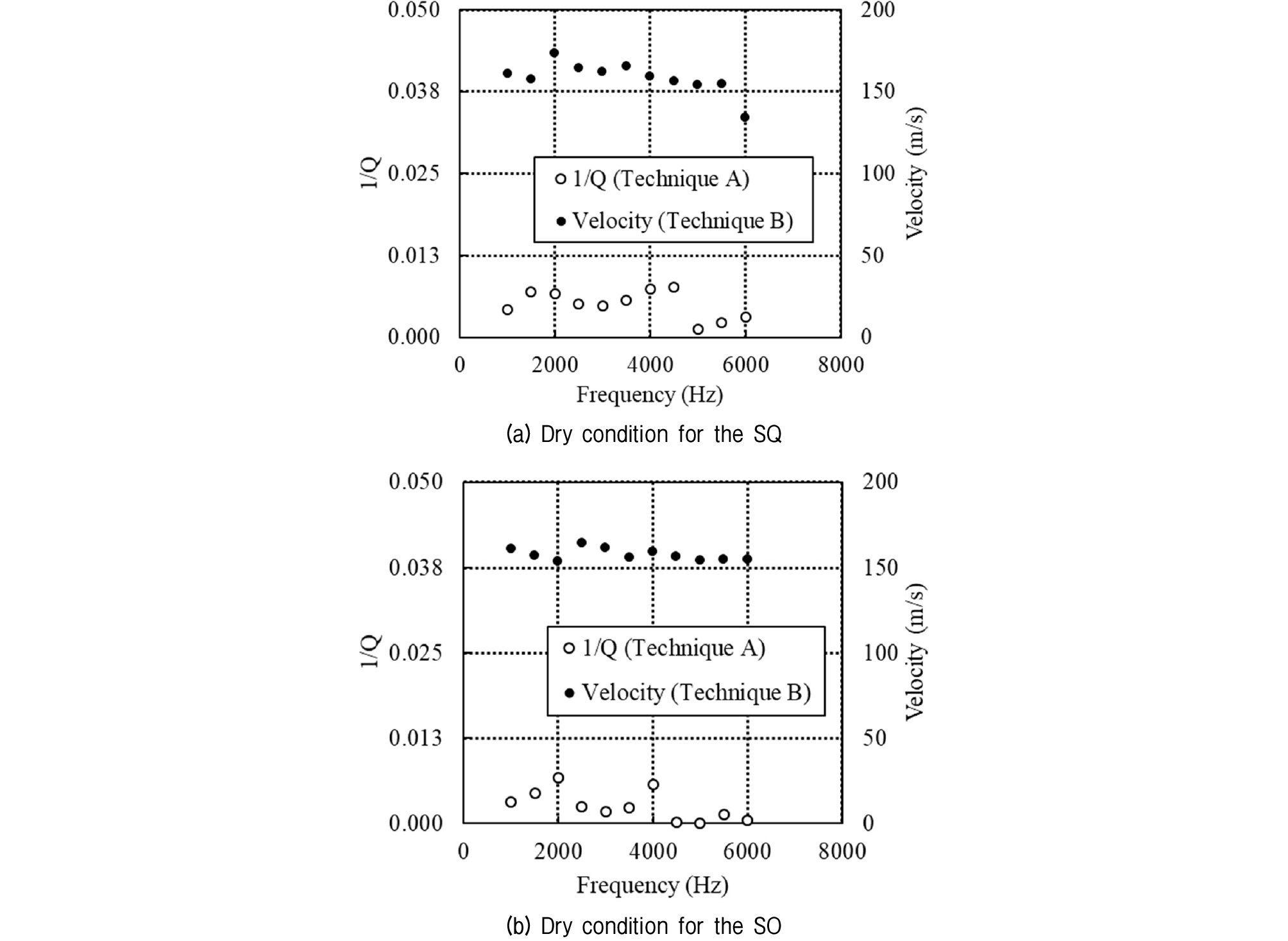
where, Vp,∞ and Vp,o are the maximum and minimum P-wave velocity, respectively. As stated by Santamarina et al. (2001), equation (3) is valid when the shear velocity is lower than 400 m/s. In this study, the measured P-wave velocity from the dry specimen was in approximately 160 m/s range as shown in Fig. 4. Therefore, Eqn (3) is applicable to analyze the test data.
6. Test Results
6.1 1/Q and Velocity Spectra for Dry Specimens
Dry specimens were tested prior to the saturated specimens in order to confirm that the characteristic frequency is a unique property of water saturated soils and that the measured characteristic frequency is not the response of the measurement system itself. Dry specimens in this study were prepared with air-dried sands. The water contents of SQ and SO specimens were 0.09% and 0.12%, respectively. In Fig. 4, for SQ and SO specimens, P-wave velocity values range from 160.92±3.38% m/s to 160.38±8.17% m/s. However, the magnitude of 1/Q turned out to be essentially zero due to A1 and A2 being equal in magnitude in Eqn (2).
It is apparent that P-wave velocity and 1/Q are essentially constant throughout the full frequency range. Overall, no characteristic frequency is observed, confirming that it does not exist for dry soils.
6.2 1/Q and Velocity Spectra for Saturated Sand Specimens
Techniques A and B were applied for measuring the characteristic frequency for specimens SQ and SO. The results are shown in Fig. 5.
In the case of SQ, the highest 1/Q was observed at 4500 Hz. The observed inflection point obtained via the velocity vs. frequency curve was 5000 Hz for SQ. The observed characteristic frequencies from techniques A and B were used for computing the hydraulic conductivity of the SQ specimen using Eqn (1), giving 1.29 × 10⁻⁴ m/s and 9.74 × 10⁻⁵ m/s. The corresponding result from the laboratory test was 2.01 × 10⁻⁴ m/s, showing good agreement with acoustically obtained numbers. A comparison of computed (1/Q)max values from Eqn (3) with test data is presented by the broken lines in Fig. 5, addressing that Eqn (3) results in an approximate upper limit of the measured (1/Q)max.
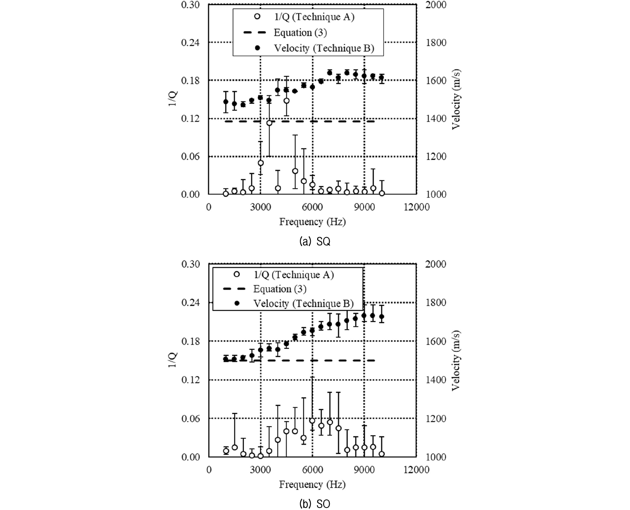
In the case of SO, the characteristic frequencies are 4.5 kHz and 6.0 kHz by techniques A and B, respectively. These frequencies resulted in hydraulic conductivities of 1.23 × 10⁻⁴ m/s and 9.28 × 10⁻⁵ m/s, while the result from the laboratory test was 1.62 × 10⁻⁴ m/s.
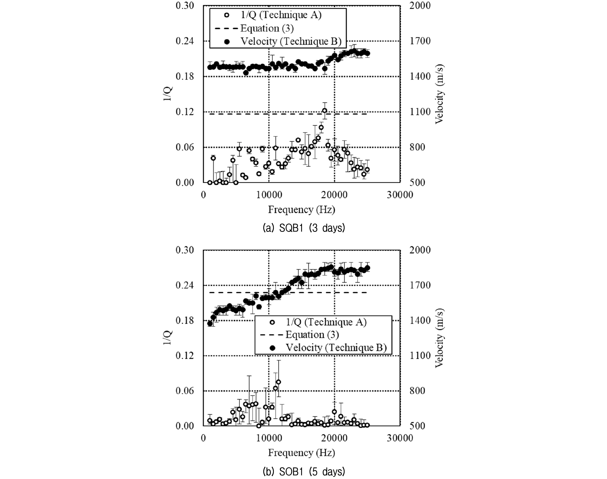
6.3 1/Q and Velocity Spectra for Saturated Sand and Bentonite Mixture
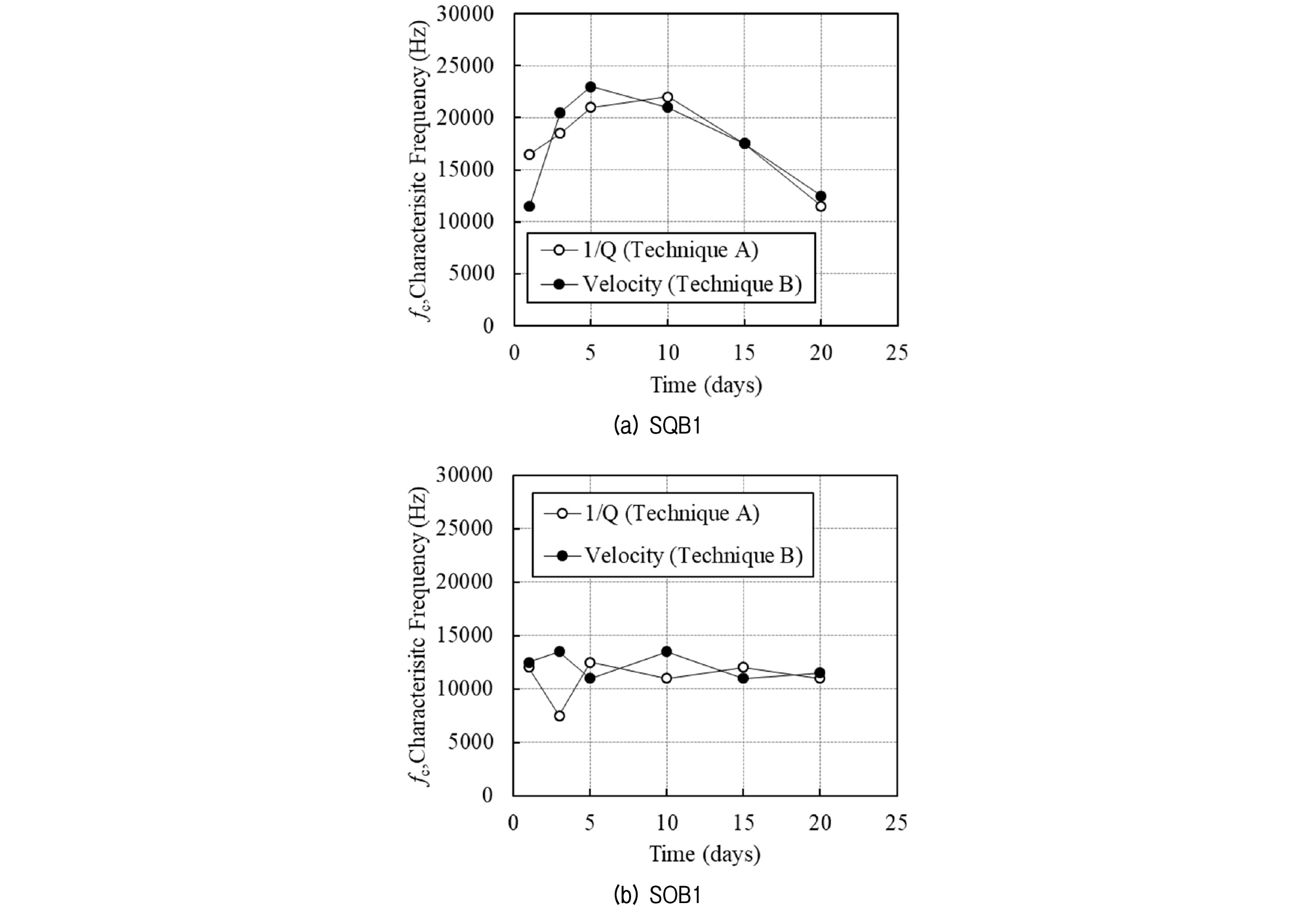
Fig. 6 shows that the overall behavior of the saturated sand and bentonite mix is similar to that of the saturated sand specimens. The computed hydraulic conductivity of SQB1 and SOB1 specimens using equation (1) and each material’s respective observed characteristic frequency—16500 Hz and 11000 Hz—turns out to be 3.36 × 10⁻⁵ m/s and 3.46 × 10⁻⁵ m/s. These numbers are comparable to the results from the laboratory tests: 4.47 × 10⁻⁵ m/s and 4.53 × 10⁻⁴ m/s, respectively. It is noted that the characteristic frequencies increased due to the reduced hydraulic conductivity from added fine material. In addition, because of the added fine material, time dependent variation of soil properties due to self-weight consolidation was expected. Acoustic measurements were made with 1, 3, 5, 10, 15, and 20 day time intervals. Figure 7 shows the variation of characteristic frequency with time for SQB1 and SOB1.
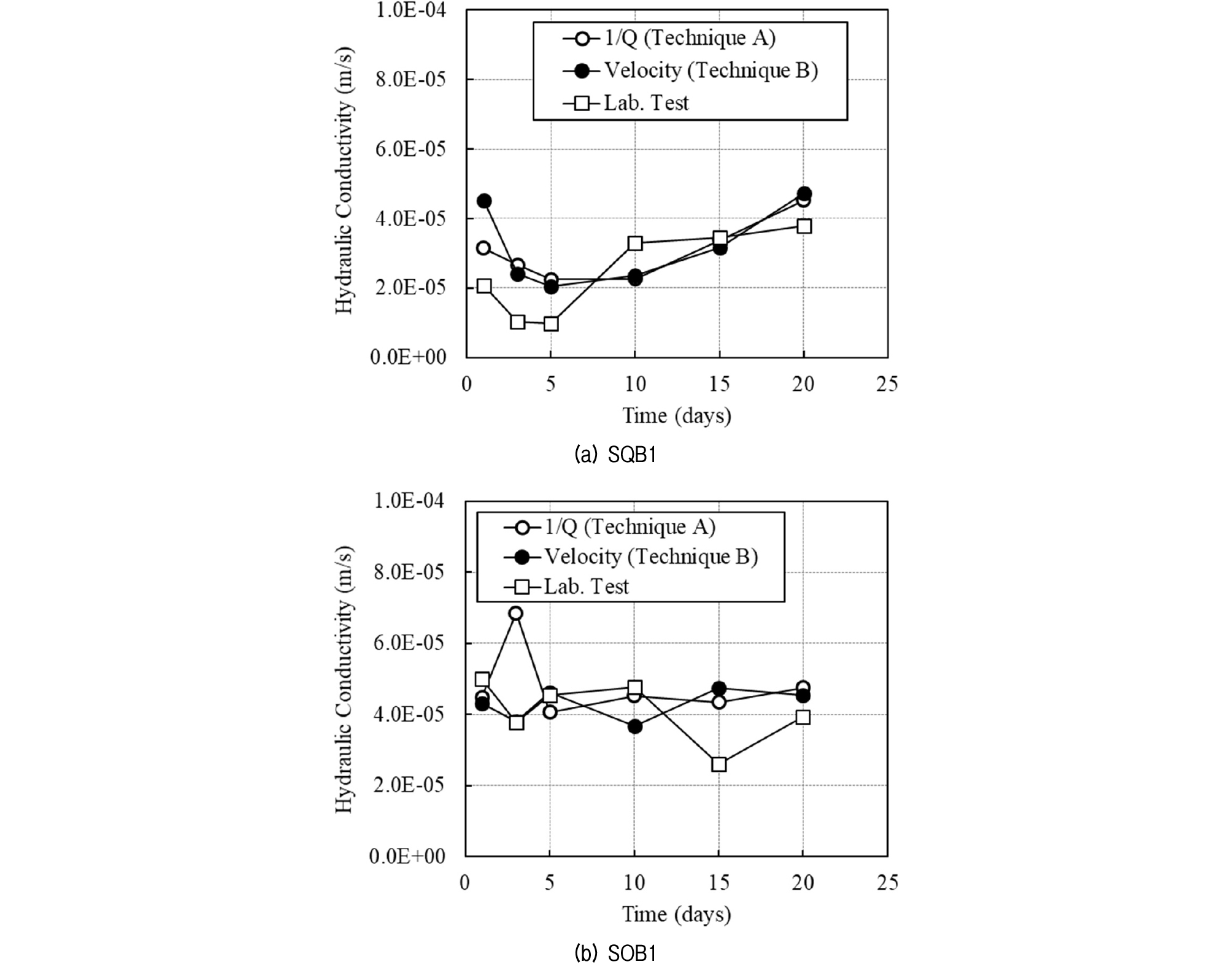
In Fig. 7, the specimen SQB1 showed noticeable variations in measured characteristic frequencies, but the sample SOB1 did not show any distinct trend. The computed hydraulic conductivities are shown in Fig. 8, demonstrating that the acoustically estimated hydraulic conductivity and the laboratory tested hydraulic conductivity vary in the same manner. The reasons why the hydraulic conductivity increases initially and then decreases later for SQB1 or why it shows more substantial changes than SOB1 are not clear. The authors postulate that this behavior is related to the stabilization process of the sand and bentonite mixture accompanied by the texture development/change as reported by Chalermyanont and Arrykul (2005). More exact analysis of this phenomenon is expected to take place in future work. Even with an imperfect understanding of the mechanisms present in Fig. 8, it is demonstrated that the acoustical technique is reliable for estimating the hydraulic conductivity of soils.
6.4 AC and DC Hydraulic Conductivity
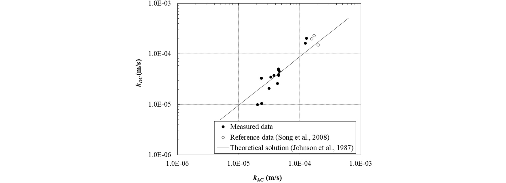
Questions may arise concerning the validity of comparing acoustically estimated hydraulic conductivity with results obtained during laboratory tests, specifically because the flow direction during an acoustic test is always alternating in a manner similar to AC electricity (soil particles move back and forth causing relative flow in pore water moving forth and back); during laboratory hydraulic conductivity tests (e.g. constant head tests), however, the flow direction is always in one direction, similar to DC electricity. In this regard, Haarten (1995) calls the hydraulic conductivity obtained from acoustic techniques the AC hydraulic conductivity, and the one obtained from traditional laboratory testing (such as a constant head testing) the DC hydraulic conductivity. The relationship between AC and DC hydraulic conductivity was proposed by Johnson et al. (1987) as follows:
where, k(ω) and k0 are the AC and DC hydraulic conductivity, respectively; ω is the angular frequency; and ωt is the transition angular frequency defined as follows:
and m is a nondimensional number (Block, 2004) given by:
where, n is the porosity, α∞ is the tortuosity, η is the dynamic viscosity of fluid, and Λ is the effective pore radius. It is also noted that the effect of the hydraulic gradient to the hydraulic conductivity was not considered in this study.
A comparison between the theoretically predicted and acoustically measured AC and DC hydraulic conductivities is shown in Fig. 9, which indicates that the real part of an AC hydraulic conductivity determined from the acoustical technique agrees fairly well with its corresponding DC hydraulic conductivity determined from traditional laboratory tests (constant head test in this study) for both the sand and the sand-bentonite mixtures. This result implies that the hydraulic conductivity obtained from the acoustic technique is theoretically and experimentally comparable to that obtained by static techniques.
7. Conclusions
The comparison of 1/Q and velocity spectra which is made in this study verifies the reliability of the acoustic technique to estimate the hydraulic conductivity of sandy soils. Two sand and two sand-bentonite mixture specimens were studied under dried and saturated conditions. The conclusions can be made as follows:
(1) 1/Q and velocity spectra are independent of the excitation frequency for the air-dried sand specimens. Therefore, the characteristic frequency does not exist for dry soils.
(2) As theoretically expected by Biot, 1/Q and velocity vary with the excitation frequencies for fully saturated specimens.
(3) Both the 1/Q and velocity spectra show the same characteristic frequency. However, velocity spectra present a more consistent characteristic frequency.
(4) The computed theoretical hydraulic conductivity using the acoustic techniques show comparable results with the conventional laboratory test results (constant head). Therefore, the implicit assumption of laminar flow in Biot’s formulation proves to be valid for sandy to silty soils.
(5) The acoustically estimated hydraulic conductivity can even trace the variation of hydraulic conductivity changes versus time for sand-bentonite mixtures.
Based on this study, the acoustic technique can be a potential alternative tool for measuring the hydraulic conductivity of sandy soils. However, further research is needed for finer silty and clayey soils.
